Forecast Module · 2026-05-01

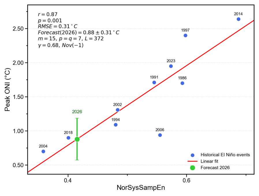
Normalized System Sample Entropy Linear Forecast Model

By Zhuomin Liu

ENSO
El Nino
ONI
NorSysSampEn
ERA5
Linear Forecast

This article presents a NorSysSampEn-based linear forecast method for the 2026 El Nino peak ONI, describing the ERA5/ONI data, preprocessing, parameter search, and model construction, and reporting the corresponding forecast results and uncertainty expression.

Forecast objective: Determine whether an El Nino event occurs in 2026; if so, forecast its peak intensity
Forecast variable: Peak ONI / Nino3.4 peak intensity
Model: Normalized System Sample Entropy linear forecast model (NorSysSampEn-based linear forecast)

Author: Zhuomin Liu

Email: zhuomin7332@163.com

References:

Meng J, Fan J, Ludescher J, et al. Complexity-based approach for El Nino magnitude forecasting before the spring predictability barrier[J]. Proceedings of the National Academy of Sciences of the United States of America, 2020, 117(1):177-183.

DOI: 10.1073/pnas.1917007117.

1. Data Overview

Raw Data

This forecast uses ERA5 reanalysis data provided by the European Centre for Medium-Range Weather Forecasts (ECMWF) for the Copernicus Climate Change Service (C3S), and takes the standardized 1000 hPa air-temperature anomaly field over the Nino 3.4 region as the base data.

For each target year, multi-gridpoint time series over the Nino3.4 region with a spatial resolution of $5^\circ\times5^\circ$ are first extracted up to the end of November or December of the previous year, and then the Normalized System Sample Entropy (NorSysSampEn) is computed.

NorSysSampEn is used to characterize the overall complexity and disorder of the climate system in the Nino3.4 region within a given time window.

This method mainly examines two precursor windows with strong linearity in the year before the forecast target year: end-November $\mathrm{Nov}(-1)$ and end-December $\mathrm{Dec}(-1)$ .

Each processed NorSysSampEn file contains the year, cutoff window, window start/end dates, and entropy value.

The entropy value is used as the input variable for the subsequent linear forecast model.

Historical training samples are the past 10 El Nino events, namely 1986, 1991, 1994, 1997, 2002, 2004, 2006, 2014, 2018, and 2023, with corresponding peak ONI values of 1.70, 1.71, 1.09, 2.40, 1.31, 0.70, 0.94, 2.64, 0.90, and 1.95.

ONI is defined as the 3-month running mean of sea-surface temperature anomalies over the Nino 3.4 region, where anomalies are based on the ERSST.v5 dataset and computed relative to a centered 30-year climatological baseline updated every 5 years.

ONI records cover the period from 1950 to the present, and can be obtained from NOAA Physical Sciences Laboratory (PSL):

https://psl.noaa.gov/data/correlation/oni.data

Data Preprocessing

We first perform leap-day removal on the raw ERA5 daily $1000\,\mathrm{hPa}$ temperature data, i.e., removing February 29 from all leap years to construct a uniform 365-day calendar.

Then, for each spatial grid point in the Nino 3.4 region, the time series are standardized by day-of-year.

Specifically, during 1979-1983, standardization for each day-of-year is based on the mean and standard deviation estimated from the fixed 1979-1983 climatology.

For 1984 and later years, standardization for a given day-of-year is based on the mean and standard deviation estimated from all available historical samples from 1979 up to that year, i.e., using an annually expanding historical baseline.

2. Forecast Algorithm and Workflow

For a detailed explanation of the System Sample Entropy method, please refer to:

This method introduces a normalized improvement to the original System Sample Entropy method, so that the tolerance parameter $\gamma$ can be fixed within a stable range, which facilitates identifying parameter intervals with high linearity.

The data window length is selected by taking data up to November 30 or December 31 of the year preceding the target forecast year and stepping backward by the effective length:

[t_{\mathrm{end}}-L+1,\,t_{\mathrm{end}}],\quad t_{\mathrm{end}}\in\{\mathrm{Nov}(-1),\,\mathrm{Dec}(-1)\}

Parameter combinations are determined jointly by the spatial asynchrony test and temporal disorder test described in the reference.

The parameter combinations are as follows:

Group	Template Length (m)	Increment Parameter (p=q)	Threshold Parameter (gamma)	Effective Length (leff)	Precursor Window
Group 1	15	7	0.30-0.80, step 0.02	99-512 days, step 7	Nov(-1), Dec(-1)
Group 2	30	15	0.60-1.00, step 0.02	75-525 days, step 15	Nov(-1), Dec(-1)
Group 3	30	30	0.60-1.00, step 0.02	90-510 days, step 30	Nov(-1), Dec(-1)
Group 4	60	15	0.70-1.10, step 0.02	75-510 days, step 15	Nov(-1), Dec(-1)
Group 5	60	30	0.70-1.10, step 0.02	90-510 days, step 30	Nov(-1), Dec(-1)
Group 6	60	60	0.70-1.10, step 0.02	120-540 days, step 60	Nov(-1), Dec(-1)

An exhaustive search is performed over different NorSysSampEn parameter combinations.

Candidate parameters include template length $m$ , time increment $p$ , extension length $q$ , similarity threshold $\gamma$ , and effective window length $L$ .

For each candidate parameter combination, NorSysSampEn values under $\mathrm{Nov}(-1)$ and $\mathrm{Dec}(-1)$ are read from the historical training samples, and the following linear model is established:

y_i=aS_i+b+\varepsilon_i,\quad i=1,2,\ldots,10

Here, $y_i$ is the peak ONI of the $i$ -th El Nino event, $S_i$ is the corresponding NorSysSampEn value in the given window, $a,b$ are regression coefficients, and $\varepsilon_i$ is the residual term.

The model is fitted using the 10 historical El Nino events, and Pearson correlation coefficient $r$ , significance level $p$ -value, and root mean square error $\mathrm{RMSE}$ are calculated.

Then, the model with the highest historical-sample correlation and lower error among all candidate parameter combinations is selected as the final forecast model.

After determining the optimal model, the NorSysSampEn value for 2026 in the same window (in practice computed from temperature data up to the end of December 2025, with lengths between 75 and 540 days) is substituted into the linear regression equation to obtain the predicted 2026 El Nino peak ONI.

Forecast uncertainty is represented by training-sample $\mathrm{RMSE}$ , so the final result is written as:

\hat{y}_{2026}=aS_{2026}+b,\qquad \hat{y}_{2026}\pm\mathrm{RMSE}

3. Forecast Results

This NorSysSampEn forecast first extracts the 2026 system sample entropy values in the two precursor windows $\mathrm{Nov}(-1)$ and $\mathrm{Dec}(-1)$ , and then searches for the optimal linear relationship in 10 historical El Nino events.

It finally outputs the optimal parameter combination, correlation coefficient, RMSE, and the predicted 2026 peak ONI.

According to the calculation results, the optimal parameter combination is:

Optimal precursor window: $\mathrm{Nov}(-1)$

Correlation coefficient in historical El Nino samples:

Root mean square error:

Substituting 2026 NorSysSampEn into the model gives the forecast peak intensity of the 2026 El Nino event as:

Overall, the NorSysSampEn forecast indicates that the ONI value forecast for 2026 based on 2025 full-year data exceeds $0.5^\circ\mathrm{C}$ , suggesting that 2026 is the onset year of an El Nino event, with a likely peak intensity of $0.88\pm0.31^\circ\mathrm{C}$ .

Researchers

Zhuomin Liu

Beijing Normal University, School of Systems Science · PhD Student
zhuomin7332@163.com
Jun Meng

Institute of Atmospheric Physics, Chinese Academy of Sciences · Distinguished Researcher / Associate Professor / Master's Supervisor
mengjun@mail.iap.ac.cn
Jingfang Fan

School of Systems Science, Beijing Normal University · Dean / Professor / PhD Supervisor
jingfang@bnu.edu.cn