Forecast Module · 2026-04-01

Enhancing the Predictability Limits of ENSO with Physics-Guided Deep Echo State Networks

By Zejing Zhang

ENSO
El Nino
DESN
ORAS5
Climate Prediction

This article presents an ENSO real-time forecasting method based on ORAS5 reanalysis data and physics-guided deep echo state networks (DESN), detailing climate-mode index construction, seasonal-cycle and trend removal, ensemble training and member selection, and reporting Niño3.4 forecast results for 2026-2027.

Forecast initialization: April 2026 | Forecast horizon: 20 months (2026-04 to 2027-12)

Model: DESN | Code: https://github.com/zhangzejing/RC-ENSO

Author: Zejing Zhang | Email: zjuer_zzj@163.com

1. Data Introduction

Raw Data

ORAS5 (Ocean ReAnalysis System 5) is operated by ECMWF and is a Copernicus C3S global ocean reanalysis product. It has a resolution of 0.25° x 0.25°, 75 vertical levels, and covers the period from 1958 to the present. The assimilation system is NEMO ocean model + NEMOVAR 3D-Var FGAT, assimilating satellite SST, sea surface height, Argo temperature-salinity profiles, and sea-ice concentration.

Official website: https://www.ecmwf.int/en/research/climate-reanalysis/ocean-reanalysis
Data access: https://cds.climate.copernicus.eu

This forecast uses two physical variables: sea surface temperature (Sea Surface Temperature, SST sosstsst) and depth of the 20°C isotherm (Depth of 20°C isotherm, D20 so20chgt). The raw data are monthly climate gridded data, with a spatial resolution of 0.25° x 0.25°, covering 1958-01 to 2026-04, with a length of 814 months.

Processed Data

1. Construct regional time series: For the two variables (Variable), the regions (Region) corresponding to each mode (mode) are spatially averaged over grid points according to the following regions. Each mode obtains one time series, with 10 time series in total, each with a time length of 814 months:

#	Mode	Full Name	Region (lat, lon)	Variable
1	Niño3.4	Niño 3.4 Index	5°S-5°N, 170°W-120°W	SST
2	WWV	Warm Water Volume	5°S-5°N, 120°E-80°W	D20
3	NPMM	North Pacific Meridional Mode	10°-25°N, 160°W-120°W	SST
4	SPMM	South Pacific Meridional Mode	25°-15°S, 110°-90°W	SST
5	IOB	Indian Ocean Basin Mode	20°S-20°N, 40°-100°E	SST
6	TNA	Tropical North Atlantic Index	5°-25°N, 55°-15°W	SST
7	ATL3	Atlantic Niño 3 Index	3°S-3°N, 20°W-0°	SST
8	IOD	Indian Ocean Dipole	(10°S-10°N, 50°-70°E) - (10°S-0°, 90°-110°E)	SST
9	SIOD	Southern Indian Ocean Dipole	(25°-10°S, 65°-85°E) - (30°-5°S, 90°-120°E)	SST
10	SASD	South Atlantic Subtropical Dipole	(40°-30°S, 30°-10°W) - (25°-15°S, 20°W-0°)	SST

2. Remove the seasonal cycle:

That is, calculate monthly anomalies. Let the original series be $X(t)$ , where $t$ denotes time and $M(t)$ denotes the corresponding month in the climatological period. The monthly anomaly is:

X'(t) = X(t) - \overline{X}_{M(t)}

where:

$X(t)$ : original value
$\overline{X}_{M(t)}$ : mean value of the series for the corresponding month in the climatological period
$X'(t)$ : monthly anomaly

The climatological period is 1979-01 to 2009-12.

3. Remove the quadratic trend:

Convert time to the monthly index $\tau(t)$ and fit a quadratic trend:

\hat{X}'(t) = a\tau(t)^2 + b\tau(t) + c

After detrending:

X''(t) = X'(t) - \hat{X}'(t)

where:

$\tau(t)$ : monthly index starting from the beginning of the series
$a,b,c$ : fitted coefficients of the quadratic trend
$\hat{X}'(t)$ : fitted trend
$X''(t)$ : monthly anomaly after removing the quadratic trend

Finally, climate-mode indices with the seasonal cycle and quadratic trend removed are obtained.

2. Forecast Algorithm and Workflow

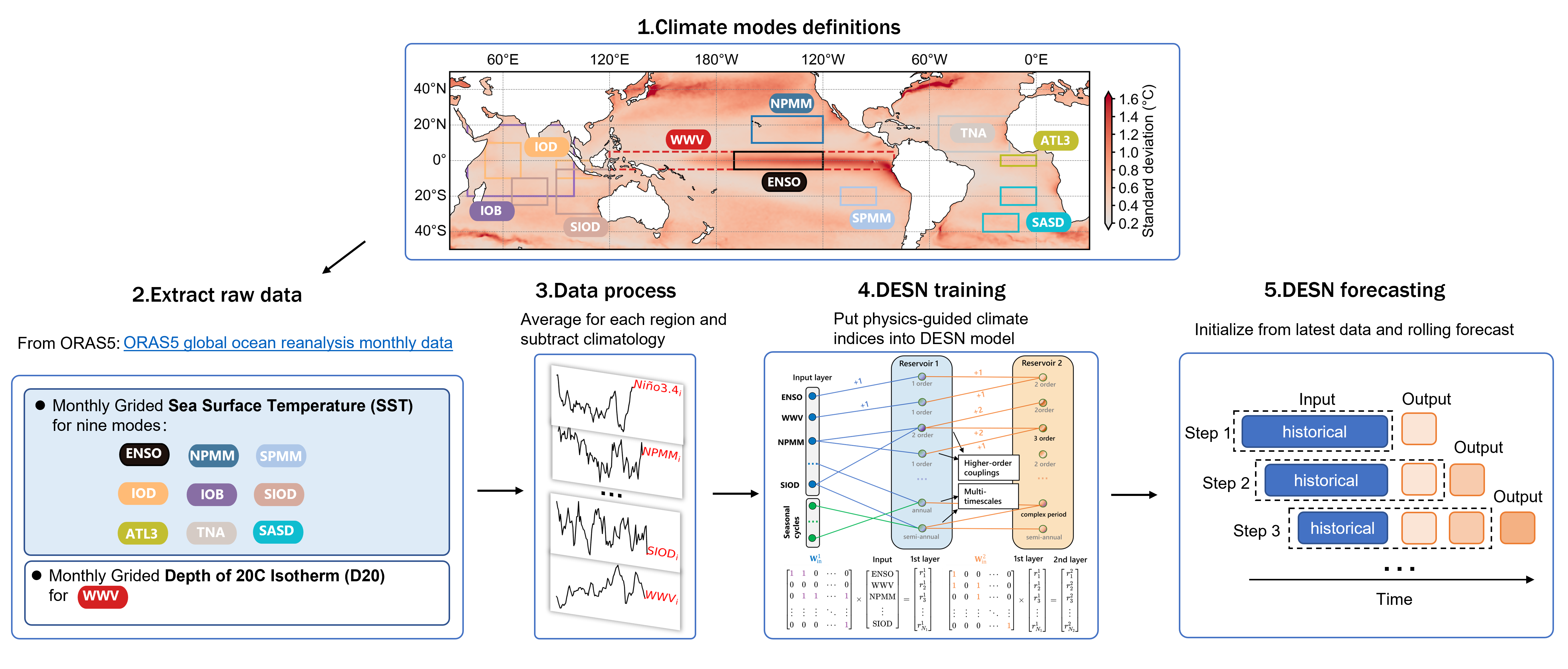
*Figure: Schematic workflow of the DESN real-time ENSO forecasting system. Climate-mode indices are extracted from ORAS5 monthly ocean reanalysis fields, including regional sea surface temperature indices and equatorial warm water volume. The processed indices are used to train the DESN model, which is then initialized with the latest available observations to produce rolling real-time forecasts.*

The 1. Climate mode definitions and 2. Extract raw data & 3. Data process steps shown in the figure have already been introduced in the first section.

The following is a brief introduction to the 4. DESN training and 5. DESN forecasting steps.

DESN is a physics-guided lightweight machine-learning forecast model. See:

Input: The climate indices introduced in the first section, together with annual-cycle and semiannual-cycle time-period encodings (Seasonal cycles).

Output: The 10 climate-mode indices for the next month. More monthly forecast results are obtained through rolling input.

Standard training and validation workflow:

Training set: 1979-2020 (504 months) | Long-term validation: 1958-1978 (252 months) | Recent validation: 2021-2026 (63 months)
Ensemble training: 5 x DESN( $n_l=1$ ) + 5 x DESN( $n_l=2$ ) = 10 members, each independently randomly initialized
Member selection: On the validation set, all combinations from C(10,4) to C(10,10) are exhaustively searched. The scoring function is the weighted Niño3.4 Pearson correlation (lead 1-15), and the optimal subset is selected
Real-time forecast: Iterative rolling. At each step, the DESN output is concatenated with the corresponding time TP encoding as the input for the next step, for a total of 20 rolling steps

3. Forecast Results

desn_forecast_2026-04

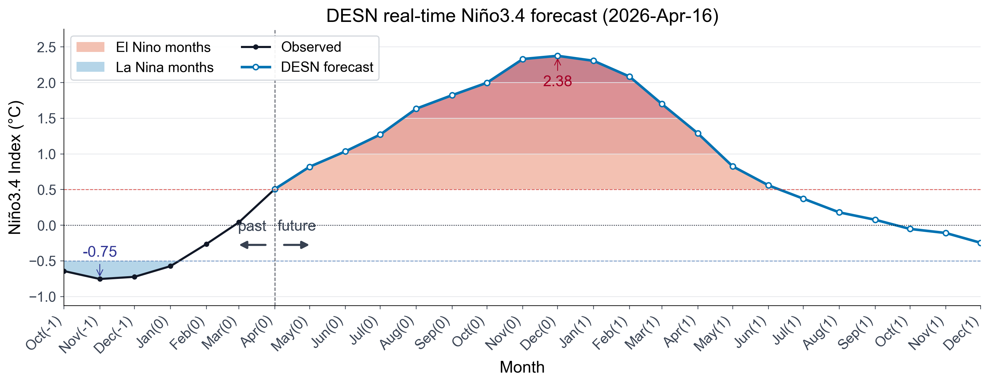
*Figure: DESN real-time Niño3.4 forecast initialized on 16 April 2026. The black curve shows the observed Niño3.4 index before initialization, and the blue curve shows the DESN ensemble-mean forecast afterward. Red and blue shading mark months exceeding the El Niño and La Niña thresholds, respectively. The vertical dashed line separates the observed past from the forecast future, and the annotated values indicate the strongest warm and cold anomalies.*

This forecast is initialized on 16 April 2026. The DESN forecast shows that the Niño3.4 index will rise rapidly from the current near-neutral warm state and exceed the +0.5°C El Niño threshold from May 2026. The ENSO signal will continue to strengthen from summer to autumn 2026 and reach its peak around December 2026, with a peak value of about +2.38°C, corresponding to a relatively strong El Niño event.

After early 2027, the warm anomaly gradually weakens and is expected to fall below the El Niño threshold around May 2027. After that, the Niño3.4 index approaches neutral and becomes slightly cold, but no clear La Niña development signal is shown within the forecast period.

Overall, the DESN forecast suggests that there is a relatively high probability of a moderate-or-stronger El Niño event in 2026-2027, with the mature phase likely occurring in winter 2026.

Researchers

Zejing Zhang

School of Physics and Technology, Beijing University of Posts and Telecommunications · Master Student
zjuer_zzj@163.com
Jun Meng

Institute of Atmospheric Physics, Chinese Academy of Sciences · Distinguished Researcher / Associate Professor / Master's Supervisor
mengjun@mail.iap.ac.cn